Some Useful Commands & Types¶

Command	Command	Command
`doc` or `help`	`clear`	`clc`
`whos`	`pwd`	`home`
`clock`	`date`	`quit`
`format short`	`format long`	`linspace( 0,1,11 )`
`sin( pi/2 )`	`sind( 90 )`	`logspace( -3,4,8 )`

MATLAB 和 Python 的区别¶

Matlab	Python
`a = 4 ^ 3`	`a = 4 ** 3`
`A = [ 1 2 3 ];`	`numpy.array([[1,2,3]])`
`~=`	`!=`
`fprintf( 'The number is %s.' , i );`	`print('The number is %s.' %i)`
末尾输入 `;` 不输出当前语句结果	没写`print`就不输出
`true` and `false`	`True` and `False`
`C:\Users\Desktop\lec\lec23.m`	`C:\\Users\Desktop\lec\lec23.py`
`zeros(3) >>>生成3*3全零数组`	`np.zeros(3) >>>生成3*1全零数组`
`mod(a,b)`	`a%b`
`%` 为comment；`#` 为脚本

Lec22-Intro¶

Numeric types¶

MATLAB numbers by default are all floats.
x = 5时，x的类型不是整数，而是双精度浮点数（double-precision floating point）

即使数值看起来像整数，它在内存中依然占用 64 位（8 字节）。
这是为了在科学计算中保持高精度并避免溢出

对于数字，MatLab实现了：

integers
floating-point numbers
complex numbers
in 8-, 16-, 32-, and 64-bit versions (like NumPy).

intN(x) & uintN(x) (N=8,16,32,64)

y_int8 = int8(x); % 转换为8位有符号整数（-128到127）
y_uint8 = uint8(x); % 转换为8位无符号整数（0到255）
浮点数转换：（不管正负号）四舍五入

matlab x = [3.7, -3.7, 2.1, -2.1]; y_int8 = int8(x); % [4, -4, 2, -2] y_uint8 = uint8(x); % [4, 0, 2, 0] 负数变为零

函数	取整逻辑	示例 (2.6)	示例 (-2.6)
`floor()`	向负无穷方向取整（地板）	`2`	`-3`
`ceil()`	向正无穷方向取整（天花板）	`3`	`-2`
`fix()`	向零方向取整（截断）	`2`	`-2`
`round()`默认	四舍五入（最接近的整数）	`3`	`-3

如果要转的数据大于类型所能承受的数据大小（如 x_int8 = int8(1000); %1000>127），则可能丢数据

whos 把workspace的所有变量的类型输出
whos a 返回a的类型

Arrays¶

A = [ 1 2 3 ];  %Python, numpy.array([[1,2,3]])
B = [ 1 2 3 ; 4 5 6 ];  %Python, numpy.array([[1,2,3],[4,5,6]])
C = [ 1 ; 2 ; 3 ];
D = [ 1 2 3 ]';  #行列转置 因此 C == D

[ 1 0 ; 0 1 ] * [ 2 2 ; 2 2 ]  % we never show this using numpy (a.dot(b))
[ 1 0 ; 0 1 ] .* [ 2 2 ; 2 2 ] % numpy a*b

eye(M,N)  #生成二维M*N数组，从（0,0）向右下角的对角线为1，其余地方为0

矩阵点乘

两个数组的每个对应维度的长度，要么相等，要么其中一个是 1
在兼容的情况下：两个数组会被自动扩展为2×3 的矩阵（取每个维度的最大长度）

D = [ 1 2 ]';     %D（2×1）广播为 2×3：`[[1,1,1]; [2,2,2]]`；
x = [ 1 0 0 ];    %x（1×3）广播为 2×3：`[[1,0,0]; [1,0,0]]`；
g = D .* x;
逐元素相乘后，g 的结果是：
[[1×1, 1×0, 1×0]; [2×1, 2×0, 2×0]] → [[1 0 0]; [2 0 0]]

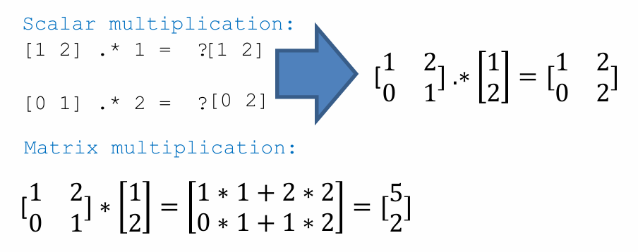
Matrix Multiplication

在MATLAB中，*运算符执行的是矩阵乘法（线性代数中的乘法），它要求：
第一个矩阵的列数 = 第二个矩阵的行数

数组的运算符

A1 = [1 2].*2    >>>[2 4] 
A2 = [1 2]*2    >>>[2 4]
C1 = [1 2].+2 -> error 
C2 = [1 2]+2    >>>[2 3]
B1 = [1 2].^2   >>>[1 4]
B2 = [1 2]^2 -> error

Array 的切片

A = [ 1,2,3 ; 4,5,6 ; 7,8,9 ];
A(2,:)    >>>[4,5,6]
A(:,2)    >>>[2,5,8]
A(2)  >>>4     %竖着数
%没有像np.array那样两个括号的取法

索引¶

从1开始，尾端取
用 () 取
a:b:c 从a开始，每次加b，直到加到>c停（不包括大于 c的）
d:e = d:1:e 即默认步长为1（从d开始加1，直到加到>e停）

1:10
1:1:10  # linspace(1,10,10)
0.1:0.1:0.5
linspace( 1,10,11 )  % np.linspace(1,10,11)
10:-1:1

用 []创造矩阵，用 ()取索引

A = [0 10 20 30 40 50 60 70 80 90 100]; 
B = A( [ 5,9,2,2 ] );
>>> [40,90,20,20]

Strings¶

msg = 'I am going to miss CS101 during my winter break!';
fprintf( msg );    #也可用 disp？

'' creates char array (字符数组)
"" creates string (字符串) 是一整个元素

s = 'I know this'
bigS = "Different? What? Confused!"   #此时bigS的length为1
s(1) >>> 'I'
bigS(1) >>> "Different? What? Confused!" %返回整个字符串
# 访问字符串内容需要使用花括号，返回字符数组
 bigS{1} >>> 'Different? What? Confused!'
 bigS{1}(1:2) >>> 'Di'

脚本(Script) & 函数(Functions)¶

脚本是用文件写成的程序。脚本文件和函数文件均带有后缀 .m

function [ output1, output2 ] = function_name( input1,input2 )
    % do what you want
end

关于 .m 文件调用函数的问题

一个 .m 文件里可以有多个函数，但只有第一个函数(主函数)能从外部访问！
第一个函数将通过 .m 文件的名称来调用

函数句柄 类似python中的单行定义函数 lambda

自定义函数：
 f = @(x) x.^2 - 1
 f(-0.5)  >>>-0.75

 如果函数是matlab自带的，那么在运行需要调用函数的工具时，前面也要加@

Loops¶

for i = 1:10
    fprintf( '%d haining',i )
end 

for i  = [char array]   #Note: char array is not string
 fprintf( '%d haining',i )
end

%% loop until condition is met
i = 0;
while i < 10
    i = i + 1;
    fprintf( 'The number is %i.' , i );
end

continue 和 break 与python中的功能一样

Logic¶

MATLAB does NOT have a bool data type.
It is called logical data type Instead of True/False, MATLAB uses integers:
0 means false; 1 means true
Recognize false and true and stores as 0 and 1
MATLAB uses 1 to indicate True, 0 to indicate False


`&` or `&&`	and
\|\| or \|	or
`~`	not

ismenber

B = [ 1 2 3 4 5 ];
ismember( 5,B ) 
>>>1

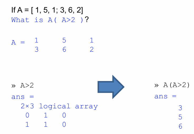
A(A>2)按照从左到右从上到下的顺序输出满足条件的元素

if a < 0
    fprintf( 'a is negative.' );
elseif a < 1
    fprintf( 'a is positive, less than unity.' );
else
    fprintf( 'a is greater than or equal to unity.' );
end

判断语句和循环语句都没有 :

Random Number Generation (`ml::rand`)¶

Distribution	Sample Commands	Meaning
uniform, `(0,1)`	`rand( 5 )`	5×5 matrix
	`rand( 5,1 )`	5×1 column vector
	`rand( 1,5 )`	1×5 row vector
	`10 * rand( 3 )`	3×3 matrix from `[0,10)`
integer, [1,n]	`randi( 5 )`	number in range `[1,5]`
最小值最后被定义	`randi( 5,2 )`	2×2 matrix with elements from `[1,5]`
	`randi( 5,[2 3] )`	2×3 matrix
	`randi( [-5,5],[10,1] )`	10×1 column vector from `[−5,−5]`
normal, μ=0, σ=1	`randn()`	normal random number
	`randn( 5 )`	5×5 matrix
	`randn( 5,2 )`	5×2 matrix
	`10 * randn( 3 ) + 5`	3×3 matrix with standard deviation 10 and mean 5

Lec23 - Input/Output¶

Save¶

A = [ 1 2 3 ; 4 5 6 ]; 
B = [ 3 4 5 ; 1 2 8 ];

M1: save( 'test', 'A' ); %save only A into 'test.mat'
or
M1: save( 'test'); %save everything in the Workspace into test.mat Or
M2: Use save test.txt A -ascii -append
to append the value of A into a file with the name test.txt

Load¶

A = load( ’test’, ’A’ ); Load variable A from text.mat
更简单的方案：双击文件，变量和值就会导入WorkSpace
A = imread( ’myPicture.jpg’ ); Use imread to open images (.jpg, .png or others) 然后用 image(); 可以输出图片

dataV = importdata( ’rainfall.txt’ );
A more advanced tool （可以处理CSVs,images,etc.）
importdata('https://zjui.intl.zju.edu.cn/sites/default/files/inline-images/WechatIMG1450.jpeg' );
无需\\, 只要 \就可以

Web I/O¶

webread processes data gracefully.

url='https://zjui.intl.zju.edu.cn/sites/defa ult/files/inline images/WechatIMG1450.jpeg' 
data = webread( url ); 
image( data );               %display image from an array (DEMO)

Plotting¶

figure(xxx) creates a new figure (window for plots).

x = 0: .1: 2*pi 
y = sin( x ) 
figure(100) %给要创建的图形一个编号 
plot( x,y,’o’ ) 
title( ’sin(x)’ ) 
xlabel( ’x values’ ) 
ylabel( ’y values’ )

[Other plots to use]:
A. fplot- 函数绘图器，无需预先生成数据点，matlab自动计算采样点

figure(1) %create a new figure numbered 1 
x = @(t) cos( 3*t ); 
y = @(t) sin( 2*t ); 
fplot( x,y ) % plot a function defined using @(t) 
hold on; %keep the graph when plotting the next

B. plot3- 绘制三维空间内曲线（曲面要用 surf 不考）

t = 0:pi/50:10*pi; 
st = sin(t); 
ct = cos(t); 
plot3(st,ct,t) % plot a 3D plot

C. fcontour- 绘制3D图的等高线

figure (2)              %create a new figure numbered 2 
f = @(x,y) sin( x ) + cos( y ); 
fcontour( f ) % plot a contour plot

D. subplot- small plots within a plot 子图布局管理器

x = linspace(0,10); 
subplot(2,1,1); % 2行1列，第1个子图
y1 = sin(x); 
plot(x,y1) 

subplot(2,1,2); % 2行1列，第2个子图
y2 = sin(5*x); 
plot(x,y2)

Single-line functions

f = @(t) 3*t;
f(3) = 9

Lec24 - Polynomial¶

Polynomial	MATLAB Representation
x+1	`[ 1 1 ]`
x	`[ 1 0 ]`
x^2+1	`[ 1 0 1 ]`
x^2+x+1	`[ 1 1 1 ]`
x^4+2x^3+3x^2+4x+5	`[ 1 2 3 4 5 ]`
5x^4+4x^3+3x^2+2x+1	`[ 5 4 3 2 1 ]`
x^6	`[ 1 0 0 0 0 0 0 ]`

polyval 用于多项式计算

polyval([ 1 2 3 4 5 ], [1,2,3]) %把x=1和2和3 带入多项式，得出含3个结果的行向量

myline = [ 1 1 ];
polyval( myline,1 );  %把x=1带入x^2+1这个多项式里

x = linspace( 0,10,101 );
y = polyval( myline,x );
figure
plot( x,y,'r-' );

myparabola = [ 2 1 1 ];
x = linspace( 0,10,101 );
y = polyval( myparabola,x );

figure
plot( x,y,'r-' );

多项式相乘用 conv

```matlab

u = [ 3 0 -1 ];
v = [ 2 5 ];

w = conv( u,v )

```matlab

polyint 多项式积分 不支持函数句柄

```matlab

integrand = [ 1 0 -1 0 ];
antiderivative = polyint( integrand );
integral_l = polyval( antiderivative,1 ); %带入端点值
integral_r = polyval( antiderivative,0 ); %带入端点值

integral = integral_l - integral_r; %作差求定积分

```matlab

数值积分 (离散点的积分

x = linspace( 0,10,11 ); 
y = [ 0.11 0.09 0.09 0.10 0.11 0.11 0.09 0.10 0.08 0.09 0.11 ]; 
figure; 
plot( x,y,’ro’ ); 
ylim( [ 0 0.2 ] );
integral = trapz( x,y );     %梯形法数值积分

polyder 多项式微分 不支持函数句柄

```matlab

polynomial = [ 1 -1 1 -1 1 -1 ];
derivative = polyder( polynomial );

```matlab

零点与极值¶

roots([]) 在多项式中找到根（包括复根），并返回为列向量

poly() 取多项式方程的根，然后将其转换回多项式数组
poly( [ 1 -1 0.5 ] )

fzero() 寻找一个函数（不一定是多项式）的零点

f = @(x) x.^2 - 1
or
f = @(x) polyval([1,0,-1], x);  %f要以函数句柄形式封装
a.fzero()
x = fzero( f,x0 )   %一个x0只能得到一个root

Minimize¶

x =-1:.01:2; 
y = humps( x ); % a function available in MATLAB 
xstar = fminbnd( @humps,0.3,1 );              %从[0.3,1] get x-value only 

OR 

[ xstar, ystar ] = fminbnd( @humps,0.3,1 );   %get x- and y-values 
figure; 
plot( x, y, xstar, ystar, ‘ro’ ); 
xlabel( ’x’ ); 
ylabel( ’f(x)’ ); 
grid on;

Lec25 - Basic Statistics¶

Statistical quantities¶

rng( 101 );    % seed the random number generator, so the set of random numbers can be always the same. Mostly for troubleshooting.
x = linspace( 0,2*pi,101 )’; 
y = x/50 + 0.002 * randn( 101,1 ); 
figure 
plot( x,y,’.’ );

mean() 平均数
medium() 中位数
Std() 标准差

x = [1 2 3 4 5];
sort(x,'descend')  >>>[5 4 3 2 1]    %默认是升序(‘ascend’)

A = [ -5 0 10 ; -3 1 9 ; -4 2 8 ; -1 3 7 ; -2 4 6 ] 
sort( A )    % 每一列从上到下升序(默认)

sort( A, 1 ) % 每一列从上到下升序(默认)

sort( A, 2 ) % 每一行从左到右升序(默认)

sortrows( A, [1] ) % 按每一行的第1个元素(默认为1)重排行 

sortrows( A,3 )% 按每一行的第3个元素重排行

matlab里把新生成的都赋给 ans ，因此原变量A不变

以上A均不变！

x = [ 1 2 3 4 5 ]; 
sum( x ) >>> ans = 15
cumsum( x ) >>>ans = 1 3 6 10 15    % 求Sn

boxplot()

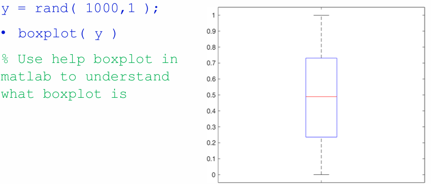
箱体的底边和顶边分别对应数据的第25百分位数（Q1） 和第75百分位数（Q3），箱子中间的标记（一条线或一个符号）代表中位数

Interpolation 插值法¶

interp1(x,y,x0,[type]) %默认为 linear，用线段穿过每两个数据点
注意，interp1() 是数字 1不是字母小写 l type 有linear(default) ,nearest,pchip/cubic`这三种

x = linspace( 0,1,11 ); 
y = x .^ 2; 
plot( x,y,’ro-’ ); 

% Get value of y at x_est 
x_est = 0.15; 
y_est = interp1( x,y,x_est ); 
hold on;
plot( x,y,’ro-’ );
plot( x_est,y_est,’bo’ );

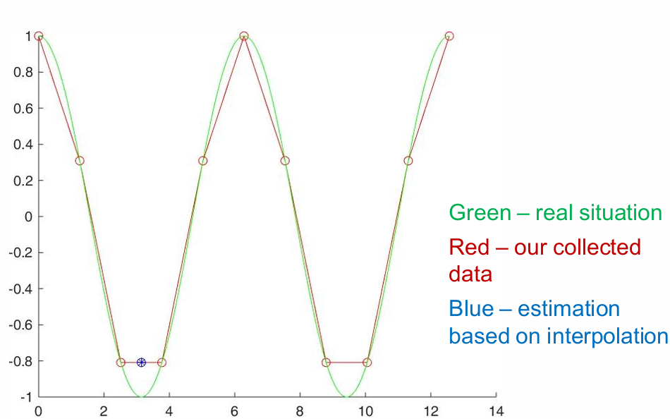
nearest 使用实际数据中最接近所需x点的x值来获得y估计值 如果是 .5，则往左取

pchip / cubic 在每两个相邻已知点之间构建一个三次多项式（除了两个数据点，还用到了这两个端点的导数（由更多点计算而来），4 个条件锁定 4 个参数，才得到唯一的三次多项式）

Matrix Equations¶

定义¶

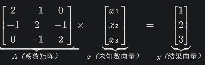
A*x = y

A：系数矩阵 → 把所有方程的 “系数” 按规则排成表格（比如 2 个方程的系数就排成 2 行）；
x：未知数向量 → 所有要解的未知数（比如 x₁、x₂、x₃）排成一列；
y：结果向量 → 所有方程等号右边的数值（比如 1、2、3）排成一列。

解法¶

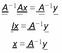
1.逆矩阵法（`x = inv(A) * y`）——类比倒数求解缺点：效率低¶

矩阵里没有 “除法”，但有类似 “倒数” 的东西叫 逆矩阵（记为 A⁻¹），满足：A * A⁻¹ = I（I 是单位矩阵，相当于矩阵里的 “1”）

所以对矩阵方程 A*x = y 两边同时乘 A⁻¹：

A = [2 -1 0; -1 2 -1; 0 -1 2];  % 3行3列，对应3个方程的系数
y = [1; 2; 3];                   % 3行1列，对应方程右边的结果

% 用逆矩阵求解
x = inv(A) * y;  % inv(A) 就是求 A 的逆矩阵

2. 左除法（`x = A \ y`）——MATLAB推荐，更高效¶

Time Code¶

tic; [operation]; toc

Lec26-Polyfit¶

Given n+1 number of ( x,y ) points (or more), we can fit a nth order polynomial as a possible curve.
polyfit(x,y,n)
p = polyfit(x,y,n) 得到从左到右an到a0的n+1个元素的行向量

%generate our x and y data 
x = rand( 5,1 ); y = rand( 5,1 ); 

%generate our fit 
xf = 0:0.01:1; 
pf1 = polyfit( x,y,1 ); %linear regression (线性回归模型)

pf3 = polyfit( x,y,3 ); %cubic 

%Plot our fit 
yf1 = polyval( pf1,xf ); 
yf3 = polyval( pf3,xf ); 
hold on 
plot( x,y,’ro’, xf,yf1,’b-’, xf,yf3,’k-’ );

% we can ask for input from user 
n = input( ’Give a polynomial order’ ); 
x = rand( n-1,1 ); 
y = rand( n-1,1 ); 
xf = 0:0.01:1; 
n1 = n              %the polynominal order you want to fit 
pf = polyfit( x,y,n1 ); 
yf = polyval( pf,xf ); 
plot( x,y,’rx’, xf,yf,’r-’ );

If n > 点的数量, MATLAB 报错:
‘Polynomial is not unique’

n不能太高，否则会为了过所有点而 overfitting ，图像会失真

Estimate the Error of a Fit¶

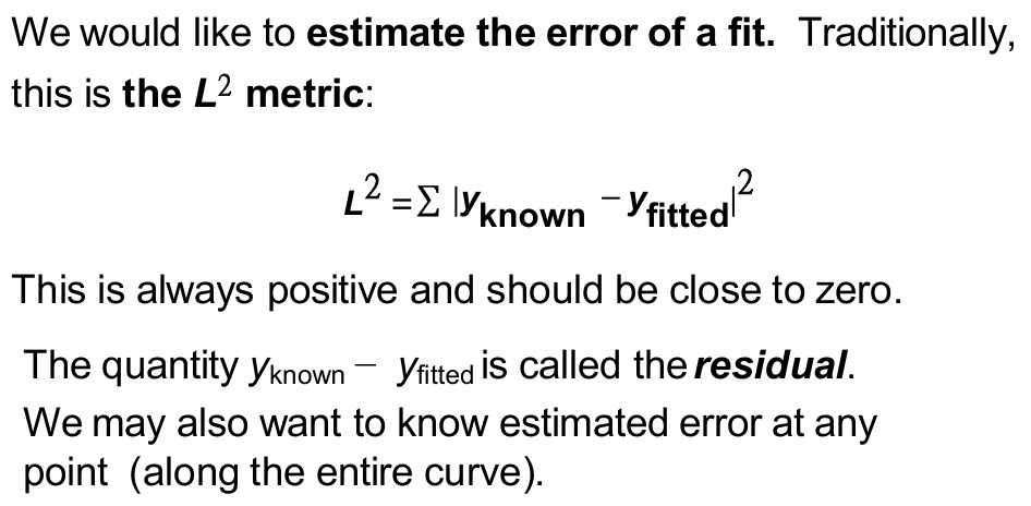
A good fit has a small residual

Another Interpolation — Spline¶

Splines 分段多项式，旨在平滑地拟合长段而不会过度拟合
Splines 通常由三多项式构成。类似 interp1() 中的 pchip
一定过所有点，因为就是取点来表示函数的

y_est = spline(x,y,x_est); %x_est => x-points you want

overshoot（过冲）
underfitting（欠拟合）

Some Useful Commands & Types¶

MATLAB 和 Python 的区别¶

Lec22-Intro¶

Numeric types¶

Arrays¶

索引¶

Strings¶

脚本(Script) & 函数(Functions)¶

Loops¶

Logic¶

Random Number Generation (ml::rand)¶

Lec23 - Input/Output¶

Save¶

Load¶

Web I/O¶

Plotting¶

Lec24 - Polynomial¶

零点与极值¶

Minimize¶

Lec25 - Basic Statistics¶

Statistical quantities¶

Interpolation 插值法¶

Matrix Equations¶

定义¶

解法¶

1.逆矩阵法 （x = inv(A) * y）——类比倒数求解 缺点：效率低¶

2. 左除法（x = A \ y）——MATLAB推荐，更高效¶

Time Code¶

Lec26-Polyfit¶

Estimate the Error of a Fit¶

Another Interpolation — Spline¶

Random Number Generation (`ml::rand`)¶

1.逆矩阵法（`x = inv(A) * y`）——类比倒数求解缺点：效率低¶

2. 左除法（`x = A \ y`）——MATLAB推荐，更高效¶